
File:Equipotential by Zureks.png

本预览的尺寸:366 × 600像素。 其他分辨率:146 × 240像素 | 639 × 1,047像素。
原始文件 (639 × 1,047像素,文件大小:111 KB,MIME类型:image/png)
摘要
| 描述 |
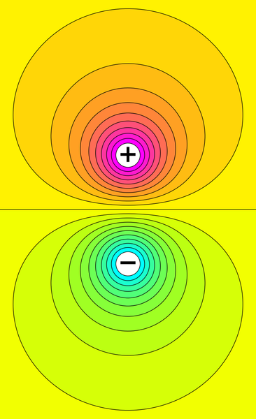
English: Voltage distribution between two electrically charged spheres (purple = positive voltage, blue = negative voltage). The black curves show equipotential contours. |
|||
| 日期 | ||||
| 来源 | 自己的作品 | |||
| 作者 | Zureks | |||
| 其他版本 |
|


Source code
The image can be created with Python Matplotlib using the following code:
import numpy as np
from matplotlib import pyplot as plt
from matplotlib import colors

cmap = colors.ListedColormap([np.clip((2*x, 2*(1-x), 4*(x-0.5)**2), 0, 1) for x in np.linspace(0., 1., 256)])

w, h = 639, 1047
xmax = 2.36
ymax = xmax * float(h) / float(w)
vmax = 0.78
y0 = 1.0
nlevels = 21
levels = np.linspace(-vmax, vmax, nlevels)
X, Y = np.mgrid[-xmax:xmax:250j, -ymax:ymax:800j]

# potential of two point charges
V  = 1.0 / np.maximum(np.sqrt(X**2 + (Y - y0)**2), 1e-2)
V -= 1.0 / np.maximum(np.sqrt(X**2 + (Y + y0)**2), 1e-2)

# rescale potential globally to make contour areas similar
V = (np.sqrt(1 + V * V) - 1) / V

plt.figure(figsize=(w/90., h/90.)).add_axes([0, 0, 1, 1])
contf = plt.contourf(X, Y, V, levels=levels, cmap=cmap,
         vmin=-vmax*(nlevels-1.)/nlevels, vmax=vmax*(nlevels-1.)/nlevels)
cont = plt.contour(X, Y, V, levels=contf.levels, colors='k', linestyles='solid')

plt.xticks([]), plt.yticks([])
plt.gca().set_aspect(aspect='equal')
plt.gca().axis('off')
plt.text(0, -y0, u'\u2212', size=48,fontweight='bold', ha='center', va='center')
plt.text(0, y0, '+', size=48,fontweight='bold', ha='center', va='center')
plt.savefig('Equipotential_of_dipole.png')
许可协议
| 本作品采用知识共享CC0 1.0 通用公有领域贡献许可协议授权。 | |
| 采用本宣告发表本作品的人,已在法律允许的范围内,通过在全世界放弃其对本作品拥有的著作权法规定的所有权利(包括所有相关权利),将本作品贡献至公有领域。您可以复制、修改、传播和表演本作品,将其用于商业目的,无需要求授权。
|
文件历史
点击某个日期/时间查看对应时刻的文件。
| 日期/时间 | 缩略图 | 大小 | 用户 | 备注 | |
|---|---|---|---|---|---|
| 当前 | 2018年5月16日 (三) 21:09 | | 639 × 1,047(111 KB) | Geek3 | Replaced with analytically computed precise contour shapes. The old version which came from an FEM simulation had significant errors towards the edges, possibly because the simulation volume was chosen too small. The potential dropped much too slowly towards the image edges. In contrast, the analytic solution is very simple, as the potential is just the linear sum of two 1/r potentials. |
| 2010年4月11日 (日) 16:37 |  | 639 × 1,047(32 KB) | Zureks | {{Information |Description={{en|1=Voltage distribution between two electrically charged spheres (purple = positive voltage, blue = negative voltage). The black curves show equipotential contours.}} |Source={{own}} |Author=Zureks |Date=2010 |
文件用途
以下页面使用本文件:
全域文件用途
以下其他wiki使用此文件:
- ar.wikipedia.org上的用途
- be-tarask.wikipedia.org上的用途
- cs.wikipedia.org上的用途
- fi.wikipedia.org上的用途
- fr.wikipedia.org上的用途
- ht.wikipedia.org上的用途
- kk.wikipedia.org上的用途
- ko.wikipedia.org上的用途
- no.wikipedia.org上的用途
- oc.wikipedia.org上的用途
- ru.wikipedia.org上的用途
- sl.wikipedia.org上的用途
- uk.wikipedia.org上的用途
- www.wikidata.org上的用途