| 描述DFT approximation to Hilbert filter.png |
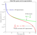
The green graph is a section of the infinitely long Hilbert transform filter impulse response. The blue graph is a shorter section, produced by the Scilab function hilb() for use as an FIR filter. hilb() apparently just applies a simple rect() window, but other windows are also possible. When the filtering (convolution) is performed by multiplication of DFTs in the frequency domain (circular convolution), people sometimes replace the DFT of hilb() with samples of the DTFT (discrete-time Fourier transform) of h[n] = 2/(πn), whose real and imaginary components are all just 0 or ±1, thereby avoiding actual multiplications. But in that case, the convolution is actually being done with the periodic summation of h[n], shown in red. Unlike hilb(), it never goes to zero, which means that the "edge effects" of circular convolution affect (distort) every output sample. They can't simply be eliminated by discarding a few corrupted samples. That effect is generally worse than the distortion caused by windowing the h[n] sequence, even with the crude rectangular window. (example) |
| Scripts InfoField | Do it in two languages (for fun).
Scilab code
N = 512;        % DFT size
L = N/2;        % length of plots
odd = 1:2:L;

// Create a segment of the IIR filter and its periodic summation
  h_IIR = zeros(1,L);
  h_periodic = zeros(1,L);
  for n = odd
    h_IIR(n) = 2/(%pi*n);
    h_periodic(n) = 2/(N*tan(%pi*n/N));      % periodic summation
  end

// Equivalent method
// M = 2*L+1;
// h_IIR = hilb(M);  //513-tap, FIR Hilbert transform filter
// h_IIR = h_IIR(L+2:M);

// Create a 65-tap, FIR Hilbert transform filter
  minimum_display_value = 0.0001;
  M = 65;
  M2 = (M-1)/2;
// The next 2 statements are equivalent to the one commented out below them
  h_65 = hilb(M);
  h_65 = [h_65(M2+2:M) ones(1,L-M2)*minimum_display_value];   // align with h_IIR
//h_65 = [h_IIR(1:M2)  ones(1,L-M2)*minimum_display_value];   // align with h_IIR

// Create another filter (equivalent to h_periodic) by sampling the DTFT
  H_DFT = %i*[0 -ones(1,L-1) ones(1,L)];
  h_DFT = real(fft(H_DFT, 1));    // inverse FFT
  h_DFT = h_DFT(2:$);             // align with h_IIR

// Display the results
  r=5; g=3; b=2;  // based on a call to getcolor()
  plot2d(odd', [h_IIR(odd)' h_DFT(odd)' h_65(odd)'], logflag="nl", style=[g r b],..
        rect=[0,minimum_display_value,256,1], frameflag=1, axesflag=1);

  title("Hilbert filter (green) and two approximations", "fontsize", 4);
  ylabel("impulse response (for n > 0)", "fontsize", 3);
  xlabel("n (odd values only)", "fontsize", 3);

  a = gca();
//a.box = "on";         included in frameflag=1
  a.font_size=3;        //set the tics label font size
  a.x_ticks = tlist(["ticks", "locations", "labels"], [1 51 101 151 201 251],..
  ["1" "51" "101" "151" "201" "251"]);

// Set line thickness of plots
  a.children.children.thickness=3;

// This works too
//f = gcf();
//f.children.children.children.thickness=3;

// Can do it this way when the thicknesses are not all the same:
// pb = a.children.children(1);    // Note that the order (compared to "style") is LIFO
// pr = a.children.children(2);
// pg = a.children.children(3);
// pg.thickness = 3;
// pr.thickness = 3;       // equivalent to set(pr,'thickness',3);
// pb.thickness = 3;
Now do it in Octave.
Octave code
pkg load signal
  N = 512;        % DFT size
  L = N/2;        % length of plots
  odd = 1:2:L;

% Create a segment of the IIR filter and its periodic summation
  h_IIR = zeros(1,L);
  h_periodic = zeros(1,L);
  for n = odd
    h_IIR(n) = 2/(pi*n);
    h_periodic(n) = 2/(N*tan(pi*n/N));      % periodic summation
  endfor

% Create a 65-tap, FIR Hilbert transform filter
  minimum_display_value = 0.0001;
  M = 65;
  M2 = (M-1)/2;
  h_65 = [h_IIR(1:M2)  ones(1,L-M2)*minimum_display_value];   % align with h_IIR

% Create another filter (equivalent to h_periodic) by sampling the DTFT
  H_DFT = i*[0 -ones(1,L-1) ones(1,L)];
  h_DFT = real(ifft(H_DFT));        % inverse FFT
  h_DFT = h_DFT(2:end);             % align with h_IIR

% Display the results
  figure
  semilogy(odd', h_IIR(odd)', 'color', 'green', 'linewidth', 2)
  hold on
% The next two statements are eqivalent
  semilogy(odd', h_DFT(odd)', 'color', 'red', 'linewidth', 2)
% semilogy(odd', h_periodic(odd)', 'color', 'red', 'linewidth', 2)

  semilogy(odd', h_65(odd)', 'color', 'blue', 'linewidth', 2)

  xlim([0 256])
  ylim([minimum_display_value 1])
  set(gca, 'xtick', [1:50:251]);

  title("Hilbert filter (green) and two approximations", "fontsize", 14);
  ylabel("impulse response (for n > 0)", "fontsize", 12);
  xlabel("n (odd values only)", "fontsize", 12);
|


![{\displaystyle \color {OliveGreen}{\boldsymbol {h[n]={\frac {2}{\pi n}}}}}](https://wikimedia.org/api/rest_v1/media/math/render/svg/1e0bb8295e56a0e53e40d4f6c72ff69e4f32dc3d)

![{\displaystyle \color {Red}{\boldsymbol {\sum _{m=-\infty }^{\infty }h[n-m\cdot 512]}}}](https://wikimedia.org/api/rest_v1/media/math/render/svg/2c57b44917a7cee58316c1c542f9375d104f09e2)