
File:Karmarkar.svg

此SVG文件的PNG预览的大小:720 × 540像素。 其他分辨率:320 × 240像素 | 640 × 480像素 | 1,024 × 768像素 | 1,280 × 960像素 | 2,560 × 1,920像素。
原始文件 (SVG文件,尺寸为720 × 540像素,文件大小:43 KB)
摘要
| 描述 |
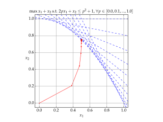
English: Solution of example LP in Karmarkar's algorithm.
Blue lines show the constraints, Red shows each iteration of the algorithm. |
| 日期 | |
| 来源 | 自己的作品 |
| 作者 | Gjacquenot |
许可协议
我,本作品著作权人,特此采用以下许可协议发表本作品:
本文件采用知识共享署名-相同方式共享 4.0 国际许可协议授权。
- 您可以自由地:
- 共享 – 复制、发行并传播本作品
- 修改 – 改编作品
- 惟须遵守下列条件:
- 署名 – 您必须对作品进行署名,提供授权条款的链接,并说明是否对原始内容进行了更改。您可以用任何合理的方式来署名,但不得以任何方式表明许可人认可您或您的使用。
- 相同方式共享 – 如果您再混合、转换或者基于本作品进行创作,您必须以与原先许可协议相同或相兼容的许可协议分发您贡献的作品。
Source code (Python)
#!/usr/bin/env python
# -*- coding: utf-8 -*-
#
# Python script to illustrate the convergence of Karmarkar's algorithm on
# a linear programming problem.
#
# http://en.wikipedia.org/wiki/Karmarkar%27s_algorithm
#
# Karmarkar's algorithm is an algorithm introduced by Narendra Karmarkar in 1984
# for solving linear programming problems. It was the first reasonably efficient
# algorithm that solves these problems in polynomial time.
#
# Karmarkar's algorithm falls within the class of interior point methods: the
# current guess for the solution does not follow the boundary of the feasible
# set as in the simplex method, but it moves through the interior of the feasible
# region, improving the approximation of the optimal solution by a definite
# fraction with every iteration, and converging to an optimal solution with
# rational data.
#
# Guillaume Jacquenot
# 2015-05-03
# CC-BY-SA

import numpy as np
import matplotlib
from matplotlib.pyplot import figure, show, rc, grid

class ProblemInstance():
    def __init__(self):
        n = 2
        m = 11
        self.A = np.zeros((m,n))
        self.B = np.zeros((m,1))
        self.C = np.array([[1],[1]])
        self.A[:,1] = 1
        for i in range(11):
            p = 0.1*i
            self.A[i,0] = 2.0*p
            self.B[i,0] = p*p + 1.0

class KarmarkarAlgorithm():
    def __init__(self,A,B,C):
        self.maxIterations = 100
        self.A = np.copy(A)
        self.B = np.copy(B)
        self.C = np.copy(C)
        self.n = len(C)
        self.m = len(B)
        self.AT = A.transpose()
        self.XT = None

    def isConvergeCriteronSatisfied(self, epsilon = 1e-8):
        if np.size(self.XT,1)<2:
            return False
        if np.linalg.norm(self.XT[:,-1]-self.XT[:,-2],2) < epsilon:
            return True

    def solve(self, X0=None):
        # No check is made for unbounded problem
        if X0 is None:
            X0 = np.zeros((self.n,1))
        k = 0
        X = np.copy(X0)
        self.XT = np.copy(X0)
        gamma = 0.5
        for _ in range(self.maxIterations):
            if self.isConvergeCriteronSatisfied():
                break
            V = self.B-np.dot(self.A,X)
            VM2 = np.linalg.matrix_power(np.diagflat(V),-2)
            hx = np.dot(np.linalg.matrix_power(np.dot(np.dot(self.AT,VM2),self.A),-1),self.C)
            hv = -np.dot(self.A,hx)
            coeff = np.infty
            for p in range(self.m):
                if hv[p,0]<0:
                    coeff = np.min((coeff,-V[p,0]/hv[p,0]))
            alpha = gamma * coeff
            X += alpha*hx
            self.XT = np.concatenate((self.XT,X),axis=1)

    def makePlot(self,outputFilename = r'Karmarkar.svg', xs=-0.05, xe=+1.05):
        rc('grid', linewidth = 1, linestyle = '-', color = '#a0a0a0')
        rc('xtick', labelsize = 15)
        rc('ytick', labelsize = 15)
        rc('font',**{'family':'serif','serif':['Palatino'],'size':15})
        rc('text', usetex=True)

        fig = figure()
        ax = fig.add_axes([0.12, 0.12, 0.76, 0.76])
        grid(True)
        ylimMin = -0.05
        ylimMax = +1.05
        xsOri = xs
        xeOri = xe
        for i in range(np.size(self.A,0)):
            xs = xsOri
            xe = xeOri
            a = -self.A[i,0]/self.A[i,1]
            b = +self.B[i,0]/self.A[i,1]
            ys = a*xs+b
            ye = a*xe+b
            if ys>ylimMax:
                ys = ylimMax
                xs = (ylimMax-b)/a
            if ye<ylimMin:
                ye = ylimMin
                xe = (ylimMin-b)/a
            ax.plot([xs,xe], [ys,ye], \
                    lw = 1, ls = '--', color = 'b')
        ax.set_xlim((xs,xe))
        ax.plot(self.XT[0,:], self.XT[1,:], \
                lw = 1, ls = '-', color = 'r', marker = '.')
        ax.plot(self.XT[0,-1], self.XT[1,-1], \
                lw = 1, ls = '-', color = 'r', marker = 'o')
        ax.set_xlim((ylimMin,ylimMax))
        ax.set_ylim((ylimMin,ylimMax))
        ax.set_aspect('equal')
        ax.set_xlabel('$x_1$',rotation = 0)
        ax.set_ylabel('$x_2$',rotation = 0)
        ax.set_title(r'$\max x_1+x_2\textrm{ s.t. }2px_1+x_2\le p^2+1\textrm{, }\forall p \in [0.0,0.1,...,1.0]$',
                     fontsize=15)
        fig.savefig(outputFilename)
        fig.show()

if __name__ == "__main__":
    p = ProblemInstance()
    k = KarmarkarAlgorithm(p.A,p.B,p.C)
    k.solve(X0 = np.zeros((2,1)))
    k.makePlot(outputFilename = r'Karmarkar.svg', xs=-0.05, xe=+1.05)
文件历史
点击某个日期/时间查看对应时刻的文件。
| 日期/时间 | 缩略图 | 大小 | 用户 | 备注 | |
|---|---|---|---|---|---|
| 当前 | 2017年11月22日 (三) 15:34 | | 720 × 540(43 KB) | DutchCanadian | The right hand side for the constraints appears to be p<sup>2</sup>+1, rather than p<sup>2</sup>, going by both the plot and the code (note the line <tt>self.B[i,0] = p*p + 1.0</tt>). Updated the header line. |
| 2015年5月3日 (日) 19:29 |  | 720 × 540(41 KB) | Gjacquenot | Updated constraint display | |
| 2015年5月3日 (日) 19:26 |  | 720 × 540(41 KB) | Gjacquenot | Updated constraint display | |
| 2015年5月3日 (日) 19:17 |  | 720 × 540(41 KB) | Gjacquenot | Updated constraint display | |
| 2015年5月3日 (日) 18:54 |  | 720 × 540(41 KB) | Gjacquenot | User created page with UploadWizard |
文件用途
以下页面使用本文件:
全域文件用途
以下其他wiki使用此文件:
- ar.wikipedia.org上的用途
- en.wikipedia.org上的用途
- fr.wikipedia.org上的用途
- ja.wikipedia.org上的用途
- ko.wikipedia.org上的用途
- pt.wikipedia.org上的用途
- ru.wikipedia.org上的用途
- simple.wikipedia.org上的用途
- uk.wikipedia.org上的用途